The functions of Excel are built-in formulas that take cells, numbers or text and return a result. This is the ultimate guide to the 31 you will use most. Learn how to total a column, make a cell decide for you, find a value in another table and clean up messy data, with an example and a common mistake for every function. Every example was checked in Excel for Windows (Microsoft 365) before it went on the list.
We recommend that you try the functions out as you read, on our practice workbook. It holds a small order list, a lookup table, messy text and a table that looks like a PDF conversion, plus a sheet that lists what to type and what you should see for all 31 functions. Download the practice workbook (Excel).
A note on versions: most of these functions work in every recent version of Excel. XLOOKUP, FILTER, SORT and UNIQUE need Microsoft 365 or Excel 2021 or later. IFS and TEXTJOIN need Excel 2019 or later. Each of these is marked in its section. In some regions Excel uses a semicolon instead of a comma between arguments. If a formula in this guide does not work, try the semicolon.
If your table started in a PDF, PDFHaul's PDF to Excel tool turns it into a spreadsheet first. The last chapter shows which of these functions clean up a table that came out of a PDF.
The 10 functions you will use most
If you only learn ten, learn these. Each one is explained in full later in the guide.
Function | What it does | Example |
|---|---|---|
SUM | Adds up a range |
|
AVERAGE | Finds the mean of a range |
|
IF | Gives one result if a test is true and another if not |
|
COUNTIF | Counts the cells that meet a condition |
|
SUMIF | Adds up the rows that meet a condition |
|
XLOOKUP | Finds a value in one column and returns a match from another |
|
TRIM | Removes extra spaces from text |
|
LEFT | Returns the first characters of text |
|
TODAY | Returns today's date |
|
IFERROR | Replaces an error with a value you choose |
|
In this guide
Chapter 1: How to write a function without memorising the syntax
Chapter 8: How to sort, filter and remove repeats with one formula
Chapter 1: How to write a function without memorising the syntax
A function is a formula with a name. You start with an equals sign, type the name, then put the inputs, called arguments, inside brackets. In =SUM(I2:I11), SUM is the function and I2:I11 is the argument. Arguments are separated by commas. You never need to remember the order, because Excel shows it as you type.
How to do it:
Click a cell and type an equals sign, then the first letters of the function, such as
=SU. Excel lists the matching functions.Use the arrow keys to pick one and press Tab to accept it. Excel adds the opening bracket.
Type or select the cells for the arguments. A tooltip under the cell shows the arguments in order, with the current one in bold.
To insert the argument names as a reminder, type just the function name, such as
=SUM, then press Ctrl+Shift+A. Excel adds the brackets and the argument names.To browse every function by category, click the fx button next to the formula bar, or press Shift+F3.
Press Enter to finish.
Chapter 2: How to total and summarise a column in seconds
These six functions answer the first questions anyone asks about a column of numbers: how much, how many, how big and how small. The examples use the Amount column of the Orders sheet in the practice workbook.
SUM
Adds up every number in the cells you give it.
Syntax: =SUM(number1, [number2], ...)
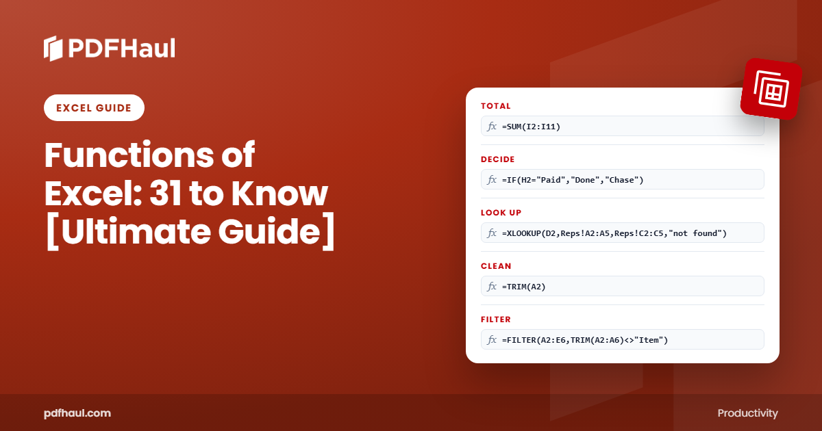
Example: Total of the Amount column on the Orders sheet. Type =SUM(I2:I11) and you should see: 379.5
Common mistake: SUM skips numbers stored as text, so a total that looks too low usually means some numbers are text. They sit on the left of the cell instead of the right.
AVERAGE
Returns the mean of the numbers in a range.
Syntax: =AVERAGE(number1, [number2], ...)
Example: Average order amount. Type =AVERAGE(I2:I11) and you should see: 37.95
Common mistake: AVERAGE ignores blank cells and text but counts zeros, so a 0 where a value is missing pulls the average down.
COUNT
Counts how many cells in a range hold a number. Dates count as numbers.
Syntax: =COUNT(value1, [value2], ...)
Example: Number of orders with a quantity. Type =COUNT(F2:F11) and you should see: 10
Common mistake: COUNT ignores text. Run it on the Note column and you get 0, even though some cells hold words.
COUNTA
Counts every cell that is not empty, whatever it holds.
Syntax: =COUNTA(value1, [value2], ...)
Example: Number of orders that have a note. Type =COUNTA(J2:J11) and you should see: 3
Common mistake: A cell that looks blank can still be counted, for example one that holds a single space or a formula that returns empty text.
MIN
Returns the smallest number in a range.
Syntax: =MIN(number1, [number2], ...)
Example: Smallest order amount. Type =MIN(I2:I11) and you should see: 22.5
Common mistake: If the range holds no numbers at all, MIN returns 0, which looks like a real answer.
MAX
Returns the largest number in a range.
Syntax: =MAX(number1, [number2], ...)
Example: Largest order amount. Type =MAX(I2:I11) and you should see: 54
Common mistake: Like MIN, MAX returns 0 when the range has no numbers, so check the range if you see 0.
Chapter 3: How to make a cell decide for you
Logic functions let a cell make a decision. They test something, such as whether an order is paid, and return a result that depends on the answer. The examples use the first row of the Orders sheet.
IF
Shows one result when a test is true and another when it is false.
Syntax: =IF(logical_test, value_if_true, [value_if_false])
Example: Label an order Done when it is Paid, and Chase when it is not. Type =IF(H2="Paid","Done","Chase") and you should see: Done
Common mistake: Text inside the formula needs quotation marks. Leave them off and Excel returns #NAME?.
IFS
Checks several tests in order and returns the result for the first one that is true. It replaces a long chain of nested IFs.
Syntax: =IFS(logical_test1, value_if_true1, [logical_test2, value_if_true2], ...)
Example: Label an order Bulk (30 or more), Standard (10 to 29) or Small. Type =IFS(F2>=30,"Bulk",F2>=10,"Standard",TRUE,"Small") and you should see: Standard
Common mistake: If no test is true, IFS returns #N/A. End with TRUE and a default value, as in the example, so there is always an answer. IFS is in Excel 2019 and later, and Microsoft 365.
AND
Returns TRUE only when every test you give it is true.
Syntax: =AND(logical1, [logical2], ...)
Example: Is the order Paid and 10 or more in quantity? Type =AND(H2="Paid",F2>=10) and you should see: TRUE
Common mistake: Write each test separately. A maths-style test such as 5<F2<30 does not work in Excel. Use AND(F2>5, F2<30).
OR
Returns TRUE when at least one of the tests is true.
Syntax: =OR(logical1, [logical2], ...)
Example: Is the order Pending or Cancelled? Type =OR(H2="Pending",H2="Cancelled") and you should see: FALSE
Common mistake: Use OR when any one test is enough and AND when all of them must pass. Mixing them up is the usual cause of a wrong result.
IFERROR
Replaces an error with a value you choose, and leaves a working result alone.
Syntax: =IFERROR(value, value_if_error)
Example: Divide the price by the quantity minus 10. For order 1001 that is a division by zero, so the formula shows a message. Type =IFERROR(G2/(F2-10),"check qty") and you should see: check qty
Common mistake: IFERROR hides every error, including real mistakes. Use it only where an error is expected, such as a lookup that may find nothing.
Chapter 4: How to count and add only the rows you want
Counting and adding only some of the rows is one of the most common jobs in a spreadsheet. These four functions do it without filtering or copying anything. The examples use the Status, Region and Amount columns of the Orders sheet.
COUNTIF
Counts the cells in a range that meet one condition.
Syntax: =COUNTIF(range, criteria)
Example: How many orders are Paid? Type =COUNTIF(H2:H11,"Paid") and you should see: 7
Common mistake: A condition with an operator needs quotation marks, such as ">=10". COUNTIF is not case-sensitive.
COUNTIFS
Counts the rows that meet two or more conditions at once.
Syntax: =COUNTIFS(criteria_range1, criteria1, [criteria_range2, criteria2], ...)
Example: How many East orders are Paid? Type =COUNTIFS(C2:C11,"East",H2:H11,"Paid") and you should see: 2
Common mistake: Every criteria range must have the same number of rows and columns.
SUMIF
Adds up the numbers in rows that meet one condition.
Syntax: =SUMIF(range, criteria, [sum_range])
Example: Total amount of Paid orders. Type =SUMIF(H2:H11,"Paid",I2:I11) and you should see: 279
Common mistake: The range to add comes last in SUMIF but first in SUMIFS. Mixing the two orders up is a common slip.
SUMIFS
Adds up the numbers in rows that meet two or more conditions.
Syntax: =SUMIFS(sum_range, criteria_range1, criteria1, [criteria_range2, criteria2], ...)
Example: Total amount of Paid orders in the West region. Type =SUMIFS(I2:I11,C2:C11,"West",H2:H11,"Paid") and you should see: 78
Common mistake: The range to add comes first in SUMIFS. All ranges must be the same size.
Chapter 5: How to find a value in another table
When the data you need sits in another table, a lookup function fetches it. XLOOKUP is the newest and easiest, so it comes first. VLOOKUP is still everywhere in older files, so it is here too. INDEX and MATCH work as a pair, or on their own. The examples use the Orders and Reps sheets.
XLOOKUP
Finds a value in one column and returns the matching value from another column. It looks for an exact match unless you change that.
Syntax: =XLOOKUP(lookup_value, lookup_array, return_array, [if_not_found], [match_mode], [search_mode])
Example: Find the rep's quota from the Reps sheet. The last argument is what to show when the rep is not found. Type =XLOOKUP(D2,Reps!A2:A5,Reps!C2:C5,"not found") and you should see: 100
Common mistake: The lookup and return ranges must be the same size. XLOOKUP is in Microsoft 365 and Excel 2021 and later, but not in Excel 2019 or earlier.
VLOOKUP
Looks down the first column of a table for a value and returns a value from a column to the right. It is older than XLOOKUP and still common in existing files.
Syntax: =VLOOKUP(lookup_value, table_array, col_index_num, [range_lookup])
Example: Find the rep's quota. The 3 means the third column of the table. FALSE asks for an exact match. Type =VLOOKUP(D2,Reps!A2:C5,3,FALSE) and you should see: 100
Common mistake: Leave out FALSE and VLOOKUP uses an approximate match, which gives wrong answers on a list that is not sorted. It can only return values to the right of the lookup column.
INDEX
Returns the value at a position inside a range.
Syntax: =INDEX(array, row_num, [column_num])
Example: The team in the third row of the Reps list. Type =INDEX(Reps!B2:B5,3) and you should see: Alpha
Common mistake: The position counts from the first cell of the range you give, not from row 1 of the sheet.
MATCH
Returns the position of a value inside a range, as a number. It is often paired with INDEX.
Syntax: =MATCH(lookup_value, lookup_array, [match_type])
Example: Position of Cara in the Reps list. Type =MATCH("Cara",Reps!A2:A5,0) and you should see: 3
Common mistake: Use 0 as the last argument for an exact match. If you leave it out, MATCH assumes the list is sorted and may return the wrong position.
Chapter 6: How to clean messy text
Text that comes from other systems, such as exports and converted files, is rarely clean. These six functions fix spaces, cut text apart and put it back together. The examples use the Text sheet and the Orders sheet.
TRIM
Removes extra spaces from text, leaving a single space between words.
Syntax: =TRIM(text)
Example: Clean the messy name on the Text sheet. Type =TRIM(A2) and you should see: Ana Smith
Common mistake: TRIM does not remove non-breaking spaces, which often come from web pages and converted files. Swap them for normal spaces first: =TRIM(SUBSTITUTE(A2,CHAR(160)," ")).
LEFT
Returns the first characters of a piece of text.
Syntax: =LEFT(text, [num_chars])
Example: The first three characters of the invoice code. Type =LEFT(B2,3) and you should see: INV
Common mistake: The result is text, even when it looks like a number, so you cannot add it up until you wrap it in VALUE.
RIGHT
Returns the last characters of a piece of text.
Syntax: =RIGHT(text, [num_chars])
Example: The last four characters of the invoice code. Type =RIGHT(B2,4) and you should see: 0042
Common mistake: A trailing space counts as a character, so a stray space at the end changes what RIGHT returns. Clean the text with TRIM first.
MID
Returns characters from the middle of a piece of text, starting where you say.
Syntax: =MID(text, start_num, num_chars)
Example: Four characters starting at the fifth character of the invoice code. Type =MID(B2,5,4) and you should see: 2026
Common mistake: The start position counts from 1, and both numbers are required.
SUBSTITUTE
Replaces one piece of text with another inside a cell.
Syntax: =SUBSTITUTE(text, old_text, new_text, [instance_num])
Example: Remove the comma from 1,234.50 in the Text sheet. Type =SUBSTITUTE(C2,",","") and you should see: 1234.50
Common mistake: SUBSTITUTE is case-sensitive. The result is still text, so wrap it in VALUE when you need a number.
TEXTJOIN
Joins text from several cells with a separator you choose.
Syntax: =TEXTJOIN(delimiter, ignore_empty, text1, [text2], ...)
Example: Join the first four reps with a comma and a space. TRUE tells Excel to skip empty cells. Type =TEXTJOIN(", ",TRUE,D2:D5) and you should see: Ana, Ben, Cara, Dev
Common mistake: The second argument is required. Forget it and the formula does not work as you expect. TEXTJOIN is in Excel 2019 and later, and Microsoft 365.
Chapter 7: How to work with dates without guessing
Dates cause more confusion than almost anything else in Excel, because they are numbers that look like text. These three functions create dates and convert them. The examples are on the Orders sheet.
TODAY
Returns today's date, and updates itself every time the workbook opens.
Syntax: =TODAY()
Example: Today's date. Format the cell as a date to read it. Type =TODAY() and you should see: Today's date (format the cell as a date)
Common mistake: Because it changes, TODAY is the wrong choice for a date you want to keep. For a fixed date, use the shortcut Ctrl+; from our Excel shortcuts guide.
DATE
Builds a date from a year, a month and a day.
Syntax: =DATE(year, month, day)
Example: March 15, 2026. Type =DATE(2026,3,15) and you should see: 46096 (shows 2026-03-15 when the cell is formatted as a date)
Common mistake: A month above 12 rolls into the next year. DATE(2026,13,1) returns January 1, 2027. That is useful on purpose and a surprise by accident.
DATEVALUE
Turns a date stored as text into a real date that Excel can sort and calculate with.
Syntax: =DATEVALUE(date_text)
Example: Convert the text 2026-03-15 into a date. Type =DATEVALUE("2026-03-15") and you should see: 46096 (same date, from text)
Common mistake: The result is a serial number until you format the cell as a date. If Excel does not recognise the text as a date, you get #VALUE!.
Chapter 8: How to sort, filter and remove repeats with one formula
These three functions are called dynamic array functions. You type one formula in one cell, and the results spill into the cells below and beside it. They need Microsoft 365 or Excel 2021 or later. In older versions they do not exist. The examples use the Orders sheet. Put each formula in an empty area, because the results need room to spill.
FILTER
Returns only the rows that meet a condition. The results spill into the cells below and beside the formula.
Syntax: =FILTER(array, include, [if_empty])
Example: All orders that are Pending. Type =FILTER(A2:I11,H2:H11="Pending") and you should see: Two rows spill out: orders 1003 and 1008
Common mistake: If something is in the way of the spill area, you get #SPILL!. With no matching rows and no third argument, you get #CALC!, so add one such as "none". FILTER is in Microsoft 365 and Excel 2021 and later.
SORT
Returns a sorted copy of a range, without changing the original.
Syntax: =SORT(array, [sort_index], [sort_order], [by_col])
Example: All orders, largest Amount first. The 9 is the Amount column, and -1 means descending. Type =SORT(A2:I11,9,-1) and you should see: Ten rows spill out, largest Amount first (order 1008, 54)
Common mistake: The sort index counts columns inside the range you chose, not the column letters on the sheet. SORT is in Microsoft 365 and Excel 2021 and later.
UNIQUE
Returns each different value once, so a repeated list becomes a list with no repeats.
Syntax: =UNIQUE(array, [by_col], [exactly_once])
Example: The regions that appear in the orders. Type =UNIQUE(C2:C11) and you should see: East, West, North (one per row)
Common mistake: East and East with a trailing space count as different values. Clean the list with TRIM first. UNIQUE is in Microsoft 365 and Excel 2021 and later.
Chapter 9: How to fix the error messages
An error message is Excel telling you what went wrong. Each one has a usual cause and a usual fix.
Error | What it usually means | How to fix it |
|---|---|---|
#N/A | A lookup did not find the value. | Check the spelling and spaces of the value you are looking for. For XLOOKUP, add a fourth argument to show a message instead. |
#VALUE! | Something in the formula is the wrong type or size, most often text where a number is expected. | Check for text in the cells. Wrap text numbers in VALUE. Make sure ranges match in size. |
#REF! | A cell the formula pointed to was deleted. | Undo the delete with Ctrl+Z, or rewrite the formula to point to the right cells. |
#DIV/0! | A number was divided by zero or an empty cell. | Check the cell you divide by. Use IFERROR if a zero is expected. |
#NAME? | Excel does not recognise a name, often a misspelt function or text without quotation marks. | Check the spelling of the function. Put text inside quotation marks. |
#SPILL! | A dynamic array formula has no room to spill, because something is in the way. | Clear the cells below and beside the formula. |
#### | The column is too narrow to show the result. | Widen the column by double-clicking the right edge of its header. |
A good habit is to read the error before you reach for IFERROR. Hiding an error does not fix the formula behind it.
Chapter 10: How to clean a table that came out of a PDF
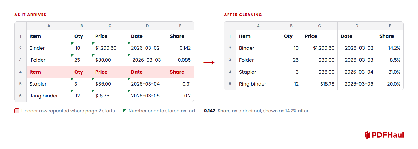
A table that comes out of a PDF often needs cleaning before you can use it. In our test of 20 PDFs and 9 tools, two problems showed up again and again. When a table runs over several pages, the header row comes back in the middle of the data, once for every page break. This happened with the three open-source libraries we tested, Camelot, Tabula and pdfplumber. And when we opened a converted file with Excel's Get Data, percentages such as 14.2% became plain numbers such as 0.142: the value was right but the percent format was gone. Two more problems, stray spaces and numbers or dates stored as text, are common in converted tables, but we did not measure them in the test. The PDF table sheet in the practice workbook contains all four, so you can try each fix.
How to do it:
Check whether the numbers are really numbers. Type
=SUM(C2:C6). You should see: 0 (every price is text, so SUM skips them)Strip the extra spaces from the text. Type
=TRIM(A2). You should see: BinderTurn the quantity into a number. Type
=VALUE(TRIM(B2)). You should see: 10Turn the price into a number. Type
=VALUE(SUBSTITUTE(SUBSTITUTE(C2,"$",""),",","")). You should see: 1200.5Turn the date text into a real date. Type
=DATEVALUE(TRIM(D2)). You should see: 46083 (2026-03-02 when formatted as a date)Remove the repeated header row. Type
=FILTER(A2:E6,TRIM(A2:A6)<>"Item"). You should see: Four rows spill out: Binder, Folder, Stapler, Ring binder
One more fix needs no function. When shares such as 0.142 should read as 14.2%, select the cells, press Ctrl+Shift+5 (Ctrl+Shift+%), then press Ctrl+1 and set one decimal place. You should see 14.2%, 8.5%, 31.0% and 20.0%. The value never changed, only how it shows. Our Excel shortcuts guide covers both shortcuts.
Once the price, quantity and date columns are real numbers and dates, SUM, SUMIFS, SORT and the other functions in this guide work on them. The price total of the four items, for example, comes to 1,285.25 after cleaning, compared with 0 before.
If you are starting from a PDF, PDFHaul's Extract Tables and PDF to Excel tools turn the table into a spreadsheet. Accuracy depends on the PDF, so check the numbers against the original, then use the steps above.
Download the practice workbook
The practice workbook has the Orders, Reps, Text and PDF table sheets used in this guide, and an Examples sheet that lists, for each of the 31 functions, where to type it, what to type and what you should see. The data is made up. Download the practice workbook (Excel)
If you liked the shortcuts side of Excel, our guide to 22 top Excel shortcuts for cleaner data covers the keyboard moves that pair with these functions.
Try one today
You do not need to learn all 31 at once. Pick one, such as SUMIF or XLOOKUP, and use it on the next table you open. If that table came from a PDF, convert it with PDFHaul first, then clean it up with the functions in Chapter 10.