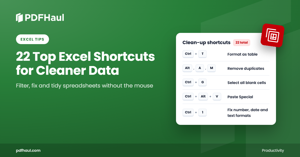
This is a list of the top Excel shortcuts for cleaning data. Learn how to fix a messy table faster, from splitting a column to selecting blanks and formatting numbers, without reaching for the mouse. Each tip gives the Windows shortcut and the Mac shortcut. The Windows shortcuts were checked in Excel before they went on the list. The Mac shortcuts come from Microsoft's documentation for Excel for Mac.
We recommend that you try these shortcuts out as you read, on our practice Excel workbook. It is a messy order list built so that you can try every tip on it. Download the practice workbook (Excel).
A note for Mac users: on a MacBook, function keys such as F2 and F4 may need the Fn key held down. Some Windows-style shortcuts, such as Ctrl+Space, can clash with default macOS keyboard settings. If one does not work, Microsoft says you can clear the matching shortcut in System Settings, under Keyboard, then Keyboard Shortcuts.
If your table started in a PDF, PDFHaul's PDF to Excel tool turns it into a spreadsheet first. These shortcuts then take it from converted to ready to use.
Get the printable cheat sheet of all 22 shortcuts at the end of this post.
In this post
1. Turn a plain range into a filterable table
Windows: Ctrl+T
Mac: Cmd+T or Ctrl+T
A range of cells is just cells. Turn it into a table and you get filter buttons, banded rows, and formulas that grow with your data. For a messy sheet, it is the fastest way to start sorting and filtering, because every column header gets its own drop-down. Tables also keep their formatting when you add new rows at the bottom, which saves cleanup later.
How to do it:
Click any cell inside your data.
Press Ctrl+T.
Check that the range shown is correct, and tick My table has headers if the first row holds column names.
Press OK. Use the filter arrows in the header row to sort or filter.
2. Remove duplicate rows in one pass
Windows: Alt, A, M
Mac: No shortcut in Microsoft's Mac list. Use the Data tab, then Remove Duplicates.
Duplicate rows quietly break totals, lookups and counts, and they are hard to spot by eye in a long table. Remove Duplicates checks the columns you choose and deletes every repeat, keeping the first row it finds. It is one of the most useful clean-up steps for exported lists and merged data. Work on a copy if you need the original, because the deletion is permanent once you save.
How to do it:
Click any cell inside your data, or select the range.
Press Alt and release it, then press A, then M. Press them one after another, not together.
In the Remove Duplicates box, tick My data has headers if the first row holds column names.
Tick the columns Excel should compare. A row counts as a duplicate only if every ticked column matches.
Press OK. Excel tells you how many duplicate rows it removed and how many unique rows are left.
3. Select every blank cell at once with Go To Special
Windows: Ctrl+G
Mac: Ctrl+G or F5
Blank cells in a table are easy to miss and slow to fix one at a time. Go To Special selects all of them in a single move, so you can fill them, mark them, or delete the rows they sit in. It is one of the quickest ways to check how complete a table really is. Select the range first, so Excel only looks at the cells you care about.
How to do it:
Select the range you want to check.
Press Ctrl+G to open the Go To box, then choose Special.
Choose Blanks and press OK. Every empty cell in the range is now selected.
Type a value, such as 0 or n/a, and press Ctrl+Enter to put it in all selected cells.
4. Paste only the values, or flip rows and columns, with Paste Special
Windows: Ctrl+Alt+V
Mac: Cmd+Ctrl+V (also Ctrl+Option+V or Cmd+Option+V)
A normal paste brings along formatting and formulas you may not want. Paste Special lets you choose exactly what comes across, which is useful when you are moving cleaned numbers into a new sheet or turning a table on its side. It is also how you lock a formula result into a plain number. Use it whenever the destination should look different from the source.
How to do it:
Copy the cells you want to move.
Click the first cell of the destination.
Press Ctrl+Alt+V to open the Paste Special box.
Choose Values to keep only the numbers and text, or tick Transpose to swap rows and columns, then press OK.
5. Select a whole block of data without dragging
Windows: Ctrl+Shift+Arrow
Mac: Shift+Cmd+Arrow key
Dragging across a long table is slow and easy to get wrong. This shortcut extends your selection to the last filled cell in the direction you choose, so one keystroke selects a whole column or row of data. Combine the Down and Right arrows to select a full table. It stops at the first blank cell, so a gap in the data will stop it early.
How to do it:
Click the first cell of the column, often the header.
Hold Ctrl and Shift, then press the Down arrow. The selection runs to the last filled cell.
Press the Right arrow while still holding Ctrl and Shift to extend across the columns.
Release the keys and apply your change, such as a format or a delete.
6. Jump to the end of a table in one key
Windows: Ctrl+Arrow
Mac: Cmd+Arrow key
Scrolling to find the last row of a long table wastes time. Ctrl with an arrow key jumps the cursor to the edge of the current block of data, so you can see how far the table runs or check the last entry. Press it again to jump to the next block. It is a quick way to confirm that nothing is missing at the bottom.
How to do it:
Click a cell inside your data.
Hold Ctrl and press the Down arrow to jump to the last filled cell in the column.
Hold Ctrl and press the Right arrow to jump to the last filled cell in the row.
Press Ctrl and the Up or Left arrow to jump back.
7. Select a full column with one shortcut
Windows: Ctrl+Space
Mac: Ctrl+Space (this one can clash with a macOS setting, see the Mac note near the top)
Clean-up often means working on a whole column, such as changing a format, widening it, or deleting it. Clicking the column letter works, but Ctrl+Space keeps your hands on the keyboard and selects the column of the cell you are in. Pair it with the insert and delete shortcuts further down this list to restructure a table without touching the mouse.
How to do it:
Click any cell in the column you want.
Press Ctrl+Space. The whole column is selected.
Apply your change, such as a format, a width, or a delete.
8. Select a full row with one shortcut
Windows: Shift+Space
Mac: Shift+Space
The same idea works for rows. Shift+Space selects the entire row of the cell you are in, which is handy for removing a repeated header row or a stray line of notes that was pulled into a table. Combined with the delete shortcut it removes a row in two keystrokes, which adds up quickly across a long sheet.
How to do it:
Click any cell in the row you want.
Press Shift+Space. The whole row is selected.
Apply your change, such as a delete, a format, or a hide.
9. Add a row or column in the right place
Windows: Ctrl+Shift++
Mac: Ctrl+Shift+= (hold Control and Shift and press the equals key)
Sometimes a table needs an extra column for a note or a calculation, or a blank row to separate groups. This shortcut inserts one where you need it. Select a whole row or column first and Excel adds it straight away. Select a single cell and Excel asks which way to shift the cells. Either way, you avoid the right-click menu.
How to do it:
Select a whole row with Shift+Space or a whole column with Ctrl+Space.
Press Ctrl+Shift++ (hold Ctrl and Shift and press the plus key).
If you selected a single cell, choose Shift cells right, Shift cells down, Entire row, or Entire column, then press OK.
10. Remove junk rows and columns fast
Windows: Ctrl+-
Mac: Cmd+- or Ctrl+-
Converted and exported tables often come with extra rows, empty columns, or repeated headers that you do not want. Ctrl+Minus deletes what you have selected. With a whole row or column selected it deletes it at once. With a single cell selected it asks how to close the gap. Use it after the selection shortcuts for a quick clean-up pass.
How to do it:
Select the row or column you want to remove, with Shift+Space or Ctrl+Space.
Press Ctrl+- (hold Ctrl and press the minus key).
If you selected a single cell, choose Shift cells left, Shift cells up, Entire row, or Entire column, then press OK.
11. Fix number, date and text formats in one box
Windows: Ctrl+1
Mac: Cmd+1 or Ctrl+1
A column that looks like numbers may be stored as text, and dates can show up in the wrong format. Ctrl+1 opens Format Cells, where you set number formats, decimal places, date styles, alignment and borders in one place. It is the first stop when a total will not add up or a date will not sort correctly, because the format controls how Excel treats the value.
How to do it:
Select the cells you want to change.
Press Ctrl+1 to open Format Cells.
Pick a tab, such as Number, Alignment, or Border, and choose your settings.
Press OK.
12. Copy a value down a column in one keystroke
Windows: Ctrl+D
Mac: Cmd+D or Ctrl+D
When many rows need the same value or the same formula, there is no need to copy and paste cell by cell. Ctrl+D copies the top cell of your selection into every cell below it in the selection, including its format. It is a quick way to repeat a category label, a unit, or a formula down a new column after you have cleaned the first row.
How to do it:
Type or fix the value in the first cell.
Select that cell and the cells below it that should match.
Press Ctrl+D. The top cell fills down through the selection.
13. Copy a value across a row in one keystroke
Windows: Ctrl+R
Mac: Cmd+R or Ctrl+R
Ctrl+R is the sideways version of fill down. It copies the leftmost cell of your selection into the cells to its right. Use it to repeat a formula across several columns, such as a total for each month, without dragging the fill handle. It also keeps the formatting, so a header style or a number format carries across the row.
How to do it:
Type or fix the value or formula in the first cell of the row.
Select that cell and the cells to its right that should match.
Press Ctrl+R. The left cell fills across the selection.
14. Repeat your last action, or lock a cell reference
Windows: F4
Mac: Cmd+T or F4 (this switches a reference between absolute and relative; Microsoft's Mac list does not give a repeat-last-action shortcut for F4)
F4 does two useful things. Outside a formula, it repeats your last action, such as a fill colour, a bold, or an inserted row, on whatever you have selected now. Inside a formula, it cycles a cell reference through its absolute and relative forms, adding the dollar signs for you. Both save repeated clicking when you are tidying a large sheet.
How to do it:
To repeat an action: do it once, such as applying a fill colour. Select another cell and press F4.
To lock a reference: click into a formula and place the cursor on a cell reference such as A1.
Press F4 to change it to $A$1. Press it again to cycle through A$1, $A1 and back to A1.
15. Fix a cell without retyping it
Windows: F2
Mac: F2, or Ctrl+U to edit with the cursor at the end of the cell
Typing over a cell replaces everything in it. F2 opens the cell for editing with the cursor at the end of the content, so you can correct a single character, trim a stray space, or adjust a formula without starting again. It is also a quick way to see the formula behind a result, which helps when you are checking numbers in a table that came from somewhere else.
How to do it:
Click the cell you want to change.
Press F2. The cursor sits at the end of the cell content.
Use the arrow keys to move to the part you want to fix, make the change, and press Enter.
16. Start a new line inside a single cell
Windows: Alt+Enter
Mac: Option+Return, or Ctrl+Option+Return
Pressing Enter normally moves you to the next cell. When a cell needs two lines, such as an address or a note, Alt+Enter starts a new line in the same cell. It keeps related text together in one cell instead of spreading it across rows. Turn on Wrap Text for the cell so both lines show.
How to do it:
Double-click the cell or press F2 to edit it.
Place the cursor where the new line should start.
Press Alt+Enter.
Press Enter to finish. Turn on Wrap Text from the Home tab if the lines do not show.
17. Format a money column as currency
Windows: Ctrl+Shift+4
Mac: Ctrl+Shift+4
A column of prices looks far clearer with a currency symbol and two decimal places, and a consistent format makes mistakes easier to spot. Ctrl+Shift+4 applies the currency format to your selection in one step. The symbol it uses comes from your computer's regional settings, so check that it matches the currency your data is in.
How to do it:
Select the cells that hold the amounts.
Press Ctrl+Shift+4.
Check the symbol and the decimal places. Use Ctrl+1 to change them if needed.
18. Format a column as percentages
Windows: Ctrl+Shift+5
Mac: Ctrl+Shift+5
A value like 0.25 means little at a glance, while 25% is clear. Ctrl+Shift+5 applies the percentage format to your selection. Remember that Excel multiplies the stored value by 100 for display, so 0.25 shows as 25%. If your numbers were already written as 25, enter them as percentages first or divide by 100, or the display will be wrong.
How to do it:
Select the cells that hold the ratios or rates.
Press Ctrl+Shift+5.
Check the result. Use Ctrl+1 to change the number of decimal places if needed.
19. Total a column or row instantly with AutoSum
Windows: Alt+=
Mac: Shift+Cmd+T
Adding up a column by hand invites mistakes. Alt+= inserts a SUM formula for the numbers next to your cell and selects the range it guessed. Check the range, press Enter, and the total is in. It is a good last step after a clean-up because it confirms the numbers add up, and a total that looks wrong can reveal a value stored as text.
How to do it:
Click the empty cell directly below a column of numbers, or to the right of a row of numbers.
Press Alt+=. Excel inserts a SUM formula and highlights the range.
Check the highlighted range, then press Enter.
20. Hide the rows you do not need
Windows: Ctrl+9
Mac: Ctrl+9 (to show the rows again, Ctrl+Shift+9)
When you only want to look at part of a table, hiding rows keeps the rest of the data intact. Ctrl+9 hides the rows of your selection. Nothing is deleted, so you can bring the rows back later. It is useful for focusing on a few records, or for hiding helper rows before you share a sheet.
How to do it:
Click a cell in each row you want to hide, or select the rows.
Press Ctrl+9. The rows are hidden.
To show them again, select the rows on either side of the hidden ones and press Ctrl+Shift+9.
21. Get back to the top of your sheet
Windows: Ctrl+Home
Mac: Ctrl+Home (on a MacBook, Ctrl+Fn+Left arrow)
After a long scroll through a big table, finding your way back is slow. Ctrl+Home takes you straight to cell A1, the top left of the sheet. It is a handy reset before you check the header row, run a filter, or start a new pass of clean-up. It pairs well with Ctrl+Arrow to move between the start and end of your data.
How to do it:
Press Ctrl+Home from anywhere on the sheet.
Your cursor moves to cell A1.
22. Stamp today's date without typing it
Windows: Ctrl+;
Mac: Ctrl+;
Logging when a table was cleaned or when a row was added is easy to forget. Ctrl+; enters today's date into the selected cell as a fixed value, so it will not change tomorrow like the TODAY function would. Use it for review dates, a last-checked column, or a note of when the data was exported.
How to do it:
Click the cell where the date should go.
Press Ctrl+; (hold Ctrl and press the semicolon key).
Press Enter. The date stays as it is.
Download the printable cheat sheet
All 22 shortcuts are on a one-page cheat sheet you can print or keep open beside your spreadsheet. Download it below.
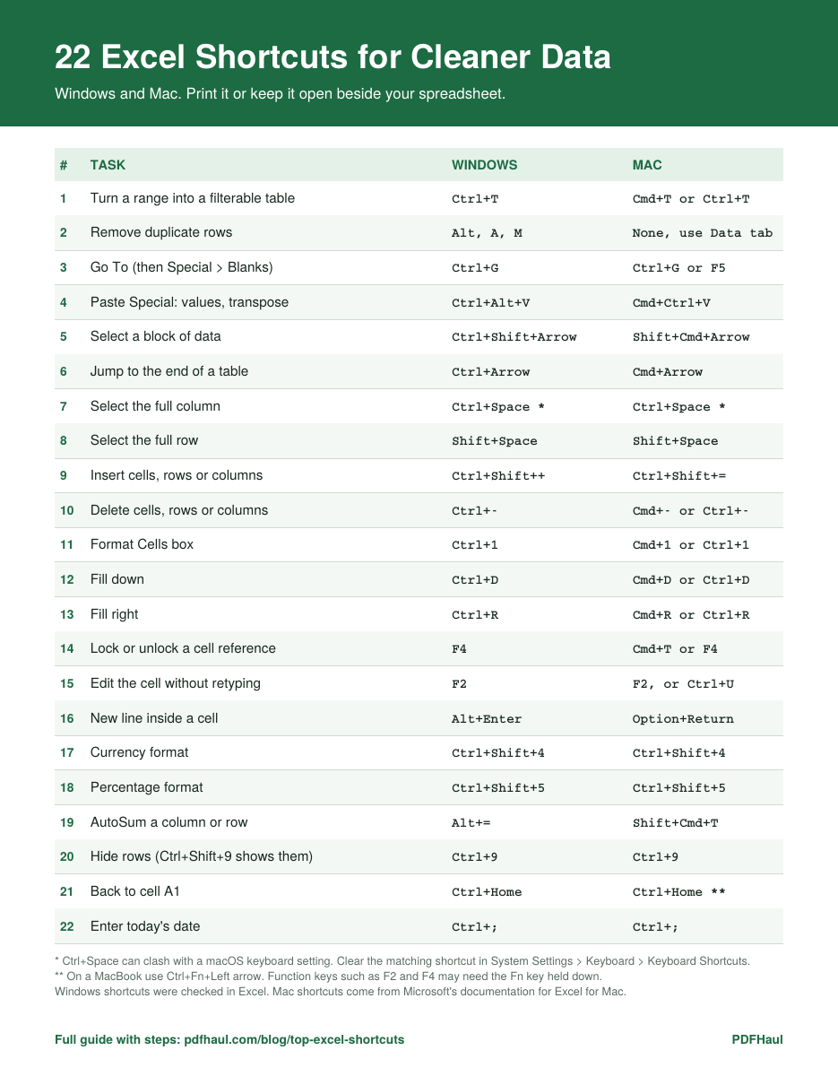
Download the cheat sheet (PDF)
The practice workbook is a messy order list with duplicate rows, blank cells, junk rows, an unused column, and dates and numbers with no formatting, plus a practice sheet for the other tips. Work through the 22 tips on it, in order. Download the practice workbook (Excel)
Try one today
You do not need to learn all 22 shortcuts at once. Pick one, such as Ctrl+T or Ctrl+G, and use it on the next table you open. If that table came from a PDF, convert it with PDFHaul first and then clean it up with the shortcut you picked.
Peter
Founder of PDFHaul and Bultech
Building tools that make working with documents faster and simpler.